1. INTRODUCTION

Flooding is one of the most widespread and damaging natural hazards worldwide, with significant impacts on human lives, infrastructure, and economic systems. Among the various types of flooding, pluvial flooding, which is caused by intense, short-duration rainfall that overwhelms surface drainage systems, has become increasingly prominent, particularly in urban environments. Unlike fluvial flooding, which is associated with river channel overflow and can often be anticipated through hydrological forecasting, pluvial floods typically develop rapidly and with limited warning. This rapid onset, combined with high spatial variability, makes pluvial flooding particularly difficult to predict and manage effectively (Bates et al., 2021).

Recent studies indicate that climate change is intensifying the hydrological cycle, leading to an increase in the frequency and magnitude of extreme precipitation events. In Central Europe, including Slovakia, several urban areas have experienced recurrent pluvial flood events in recent years, resulting in substantial economic losses and disruptions to infrastructure (Vojtek et al., 2024; 2026b). Urbanization further exacerbates the problem by increasing impervious surfaces, reducing infiltration capacity, and accelerating surface runoff. As a result, there is a growing need for reliable, high-resolution, and computationally efficient tools for mapping pluvial flood inundation to support risk assessment, urban planning, and emergency management (Rosenzweig et al., 2018).

Traditional flood modeling approaches rely on physically based hydrologic and hydraulic models (Mudashiru et al., 2021). These models simulate the underlying processes governing rainfall-runoff transformation and surface water flow, often using systems of partial differential equations such as the shallow water equations (Teng et al., 2017; Vojtek & Vojteková, 2026). While such models are capable of producing highly detailed and physically consistent results, they are computationally expensive, require significant expertise to set up and calibrate, and depend on the availability of high-quality input data (Vojtek et al., 2023b; Cea et al., 2025). Consequently, their application is often limited to small study areas or offline analyses, making them less suitable for real-time forecasting or rapid scenario evaluation (Mediero et al., 2022; Sañudo et al., 2025).

In response to these limitations, data-driven approaches, particularly those based on machine learning (ML), have gained increasing attention in the field of flood modeling. Machine learning algorithms are capable of capturing complex, nonlinear relationships between input variables and flood responses without explicitly solving physical equations (Chu et al., 2020). Once trained, ML models can generate predictions in a fraction of the time required by traditional hydraulic simulations, making them attractive for rapid flood mapping and early warning applications (Shao et al., 2024; Asif et al., 2025). Recent advances in computational power, data availability, and algorithm development have further accelerated the adoption of ML techniques in hydrological research (Bentivoglio et al., 2022; Liao et al., 2023; Vojtek et al., 2026a).

A critical aspect of applying ML to flood inundation mapping is the generation of reliable training datasets. Since observed flood data are often sparse, incomplete, or unavailable, especially for pluvial events, synthetic data derived from high-resolution hydraulic models can be used instead (Guo et al., 2021). These hydraulically derived water depths provide physically consistent representations of flood behavior under various rainfall scenarios and can serve as a robust foundation for training ML models (Sejinja et al., 2025). By learning from these simulations, ML can effectively approximate the behavior of complex hydraulic systems while reducing computational demands (Li et al., 2025).

In addition to high-quality training data, the performance of ML-based flood models strongly depends on the availability of detailed spatial information (El Baida et al., 2024). High-resolution digital elevation models (DEMs) or land use/land cover datasets play a crucial role in determining flood dynamics (Rözer et al., 2021). The integration of such high-resolution spatial data enables ML models to capture fine-scale variations in topography and surface properties, which are essential for accurately predicting inundation extent and depth in heterogeneous urban environments (Berkhahn et al., 2019; Bartlett et al., 2025).

This study proposes a ML-based framework for rapid pluvial flood inundation mapping that leverages hydraulically derived water depths and high-resolution spatial datasets. The central premise is that ML models can be trained to emulate the outputs of computationally intensive hydraulic simulations, thereby enabling computationally efficient and surrogate prediction of flood inundation under varying rainfall conditions. The framework combines physically informed training data with spatially rich input features to enhance predictive accuracy while maintaining computational efficiency.

The proposed approach is demonstrated through a case study in Slovakia, a country characterized by diverse topography and increasing exposure to extreme rainfall events. Several urban and peri-urban areas in Slovakia have experienced significant pluvial flooding in recent years, highlighting the need for improved flood mapping tools tailored to local conditions (Copernicus, 2024). The availability of high-resolution spatial data, including detailed DEM and land cover information, provides an opportunity to develop and evaluate ML-based methods for flood prediction.

The objectives of this study are as follows. First, to develop a ML model, in particular the eXtreme Gradient Boosting (XGB), capable of predicting pluvial flood inundation extent and water depth based on hydraulically derived flow depths from four rainfall scenarios and high-resolution spatial predictors. Second, to evaluate the performance and computational efficiency of the ML model using relevant quantitative metrics. By addressing these objectives, this study contributes to the growing body of research on hybrid and data-driven flood modeling approaches. It demonstrates how ML, when combined with physically based training data and detailed spatial information, can provide an alternative to traditional hydraulic models for rapid inundation mapping. 

2. MATERIALS AND METHODS

2.1. Study area

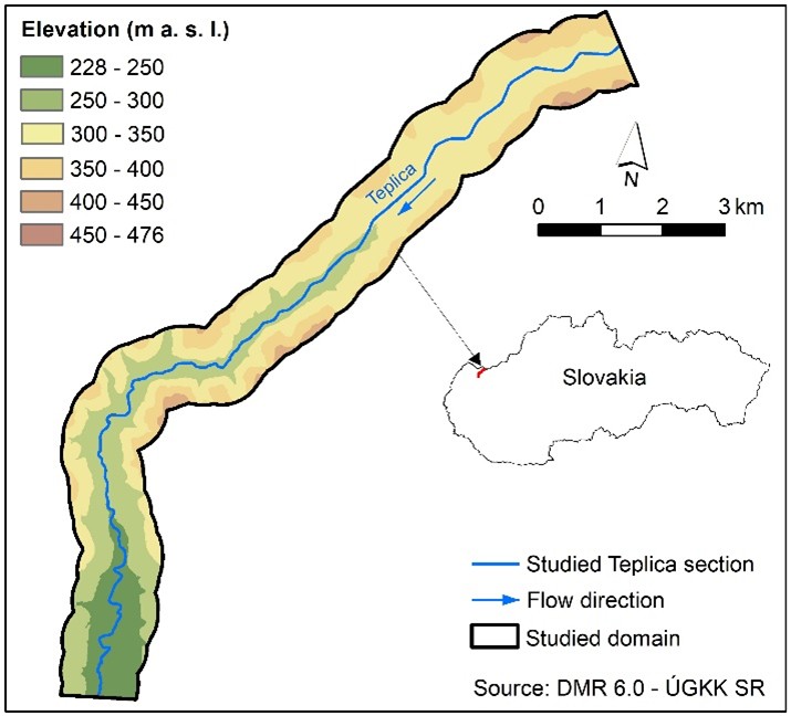
In this study, we demonstrate the application of our methodology on a domain along 17 km of the Teplica River, which is located in western Slovakia. A buffer zone of 600 m on each side of the river was created, having an extent of 19.2 km². The elevations range between 228 and 476 m a. s. l. (Figure 1).

2.2. Predictor processing

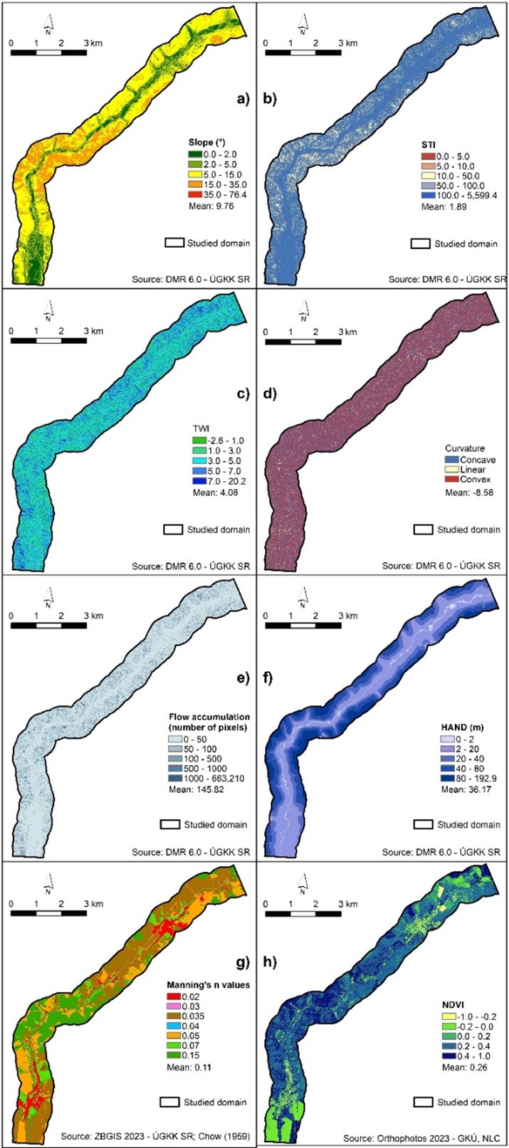
Eight physical-geographical predictors, namely, slope, curvature, sediment transport index (STI), topographic wetness index (TWI), flow accumulation, height above the nearest drainage (HAND), surface roughness, and the normalized difference vegetation index (NDVI), were selected for the ML application. 

The morphometric and hydrographic predictors (slope, curvature, TWI, STI, flow accumulation, and HAND) were processed based on the LiDAR digital elevation model (DEM) DMR6.0 with a resolution of 0.5 m. The DEM was obtained from the Geodetic and Cartographic Institute. The HAND raster was derived based on procedure described in Vojtek et al. (2025). All DEM-derived maps were generated using the ArcGIS software.

The surface roughness predictor was derived based on the Basic Data Base for Geographic Information System (ZBGIS) from 2023, which was provided by the Geodetic and Cartographic Institute. Based on Chow (1959), the following Manning’s n coefficients were assigned to individual LULC classes derived from ZBGIS 2023: built-up area (0.02), roads (0.02), railway (0.02), material/waste dump (0.03), urban greenery (0.05), forest (0.15), grassland (0.05), orchards and garden (0.07), arable land (0.035), channel (0.04), and water body (0.04). The NDVI predictor was created in ArcGIS software based on orthophotos from 2023 with 15 cm resolution. The surface roughness and NDVI were resampled to a spatial resolution of 0.5 m to ensure consistency with the DEM-derived predictors.

2.3. Multicollinearity among predictors

To reduce redundancy among input variables, a multicollinearity assessment was performed on the eight selected predictors. Both Pearson’s correlation coefficient and the variance inflation factor (VIF) were employed to quantify the level of interdependence among the predictors (Alin, 2010). Threshold values for identifying problematic multicollinearity were selected based on previous studies (Tamura et al., 2019; Vojtek et al., 2023a; Pakdehi et al., 2024). Specifically, predictors with VIF values exceeding 5 and Pearson correlation coefficients greater than 0.7 would be considered highly collinear and thus unsuitable for inclusion in the ML model.

2.4. Training the XGB-ML models 

Training datasets representing flow depths were produced using a two-dimensional (2D) hydraulic model implemented in MIKE+. For the floodplain, a triangular computational mesh was developed. The maximum element size was 9 m². The river channel was discretized separately using a quadrangular mesh, with a maximum longitudinal resolution of 5 m and a transversal resolution of 2 m to better capture channel flow dynamics. In total, the mesh for the Teplica domain comprised 3,212,971 elements, with an average element area of approximately 5.79 m². 

The XGB models were trained using pluvial flood depth maps derived from hydraulic simulations under four uniform rainfall scenarios, characterized by intensities of 20, 40, 60, and 80 mm/h. The simulations were carried out using a rain-on-grid approach, incorporating spatially variable Manning’s roughness coefficients and infiltration rates corresponding to different LULC classes. The assignment of Manning´s n roughness values was done following the work by Chow (1959) while the infiltration losses for individual land cover classes were assigned following the work by Rahmati et al. (2018). The infiltration rate for individual land cover classes was as follows: built-up area (5 mm/h), asphalt roads (1 mm/h), railway (5 mm/h), urban greenery (20 mm/h), forest (40 mm/h), grassland (30 mm/h), orchards and garden (20 mm/h), arable land (10 mm/h), channel (0 mm/h), and water body (0 mm/h). The other parameters for hydraulic modeling were set as follows. The upstream boundary condition was set to discharge (5 m3/s) while for the downstream boundary condition, it was the water level (228.9 m). Initial conditions were set as uniform water level (228.2 m). The simulation time step was set to 10 seconds, as this is a common and recommended value by DHI for detailed yet efficient simulations aiming to achieve numerical stability in the model. We used a 2D overland solver with a cell-centered Finite Volume method to solve the shallow water equations.

For the classification task, the simulated flow depth maps were converted to binary flooded/non-flooded targets based on positive flow depth. For the regression task, flow depths were min-max normalized to the [0,1] interval separately for each rainfall scenario before model training and evaluation.

To ensure robust model performance, a spatially structured 10-fold cross-validation strategy was employed during the training process (Figure 2).

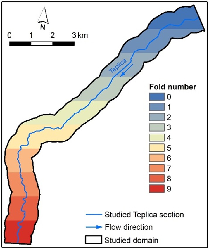
The Teplica domain was divided into ten contiguous blocks along the longitudinal direction of the domain using the y-coordinate (fold number = 0-9), rather than randomly assigning individual pixels to folds. In each cross-validation run, one complete spatial block was withheld as the test fold and the remaining nine blocks were used for training. This block-wise design provides a more rigorous test of spatial transferability than a random pixel-level split because the model has to predict an unseen spatial part of the domain.

2.5. XGB classification and regression

XGB is an ensemble learning algorithm based on gradient boosting, where decision trees are constructed iteratively to optimize a differentiable loss function. The method incorporates regularization to control model complexity and prevent overfitting (Chen & Guestrin, 2016). 

In case of our domain, separate scenario-specific XGB models were trained for the 20, 40, 60, and 80 mm/h rainfall scenarios, with hyperparameters defined individually for each scenario within each task. This modelling choice was made because the available hydraulic training data consisted of four discrete design rainfall simulations, each producing a different flood extent, class balance, and normalized depth distribution. The objective of the study was therefore to emulate the predefined design scenarios used for rapid hazard mapping, rather than to interpolate or extrapolate across a continuous rainfall-intensity space. A single rainfall-conditioned model would require a larger set of rainfall events to robustly learn the intensity-depth relationship; with only four steady-state scenarios, separate models preserve the scenario-specific hydraulic response patterns. Hyperparameters were selected empirically through preliminary sensitivity testing over a limited range of tree numbers, maximum depths, learning rates, minimum child weights, subsampling ratios, and gamma values, with the aim of improving cross-validation performance while limiting overfitting and excessive computation time. The selected values should therefore be interpreted as empirically tuned scenario-specific configurations rather than as global optima from exhaustive automated optimization. All models used the tree booster ('gbtree') with histogram-based tree construction ('hist'). Regularization parameters were kept constant across all scenarios, including L1 regularization (reg_alpha = 0.1) and L2 regularization (reg_lambda = 1.0), together with a fixed random state of 42 and parallel training on 64 CPU cores.

For classification, the 'binary:logistic' objective and log-loss evaluation metric were used, with scale_pos_weight = 1. Model configurations varied across rainfall scenarios. For the 20-mm/h scenario, the model used 1000 trees with a maximum depth of 8, learning rate of 0.03, and minimum child weight of 4. For 40 mm/h, 900 trees were used with depth 7, learning rate 0.02, and minimum child weight 8. For 60 mm/h, the configuration was reduced to 800 trees, depth 6, learning rate 0.01, and minimum child weight 10. For 80 mm/h, the model used 600 trees with depth 6, learning rate 0.01, and minimum child weight 25. Subsampling parameters were set to 0.85 for both row and column sampling in the 20 and 40 mm/h scenarios, and to 0.80 in the 60 and 80 mm/h scenarios. The gamma parameter was set to 0.5 for 20 mm/h and 1.0 for the remaining scenarios.

For regression, the same configuration strategy was applied using the 'reg:logistic' objective. Compared to classification, the number of boosting rounds was increased, with 1200 trees for 20 mm/h, 1100 for 40 mm/h, 1000 for 60 mm/h, and 800 for 80 mm/h while all other hyperparameters remained consistent with the classification settings. The 'reg:logistic' objective was used deliberately because the regression target values were min-max normalized to the [0,1] interval separately for each rainfall scenario. In this application, the objective was therefore used to constrain predicted normalized depths to the same bounded interval, not to predict flood probabilities. The resulting predictions were evaluated against the corresponding normalized hydraulically simulated flow depths. Although reg:squarederror is more commonly used for continuous depth regression problems, reg:logistic was selected in this study because the target values were normalized to the [0,1] interval, allowing predictions to remain constrained within the same bounded range.

The XGB models were computed on the following hardware: CPU: AMD EPYC 7542 32-Core Processor, architecture: x86/64, type of CPU: Server (EPYC, Zen 2 architecture), physical cores: 32, logical cores: 64 using simultaneous multithreading, number of sockets: 2, basic frequency: 2.9 GHz, maximum boost frequency: 3.35 GHz, L2 Cache: 16 MB, L3 Cache: 128 MB.

2.6. Performance of XGB model

The XGB classification of pluvial flood extent was evaluated using Recall, Precision, and F1-score while the performance of XGB regression of water depths was assessed using the root mean square error (RMSE), mean absolute error (MAE), and Bias. Because the regression target was min-max normalized separately for each rainfall scenario, RMSE, MAE, and Bias were calculated on the normalized [0,1] scale and are reported as dimensionless percentages of the scenario-specific hydraulic depth range. Since the minimum simulated depth in each scenario was zero, these percentages are effectively relative to the maximum simulated depth for the given rainfall scenario.

3. RESULTS AND DISCUSSION

3.1. Training data from hydraulic model

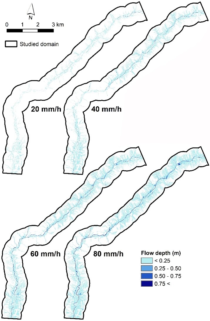
Figure 3 shows the hydraulically modeled flow depths, which were generated after applying the rain-on-grid method in the MIKE+ model for four studied rainfall scenarios (20, 40, 60, and 80 mm/h).

3.2. Multicollinearity

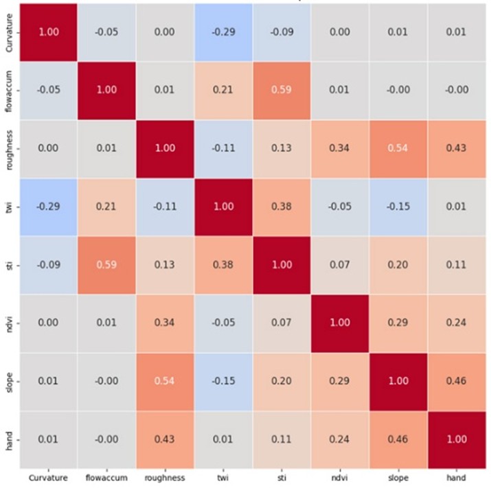
Figure 4 presents the Pearson correlation coefficients calculated among the selected predictors. None of the predictors exceeded the predefined correlation threshold of 0.7, indicating an absence of strong pairwise linear relationships. The highest positive correlation was observed between STI and flow accumulation (0.59), followed by the relationship between the roughness and slope (0.47).

The multicollinearity assessment based on VIF further confirmed these findings, as all predictors exhibited values below the critical threshold of 5 (Table 1). The largest VIF values were associated with STI (1.92) and slope (1.72), though these remain well within acceptable limits. Overall, the results indicate that the selected predictors do not exhibit problematic multicollinearity and can be considered sufficiently independent for ML modeling.

3.3. Maps of predictors

Figure 5 illustrates the spatial distribution of predictors used in ML modeling for the Teplica domain. The mean slope in this area reaches 9.76° (Figure 5a), indicating relatively moderate terrain gradients. The mean STI value is 1.89 (Figure 5b), suggesting a relatively low potential for concentrated surface runoff and erosive processes. The TWI exhibits an average value of 4.08 (Figure 5c), reflecting moderate moisture accumulation conditions across the domain. Curvature map with mean value of -8.58 is presented in Figure 5d, indicating a predominance of concave terrain features. Flow accumulation is shown in Figure 5e with the mean value of 145.82. The HAND map shows a mean value of 36.17 m (Figure 5f). The mean NDVI value for the Teplica domain is 0.26 (Figure 5h), indicating moderate vegetation density across the study area.

3.4. ML-based flood extent and water depths

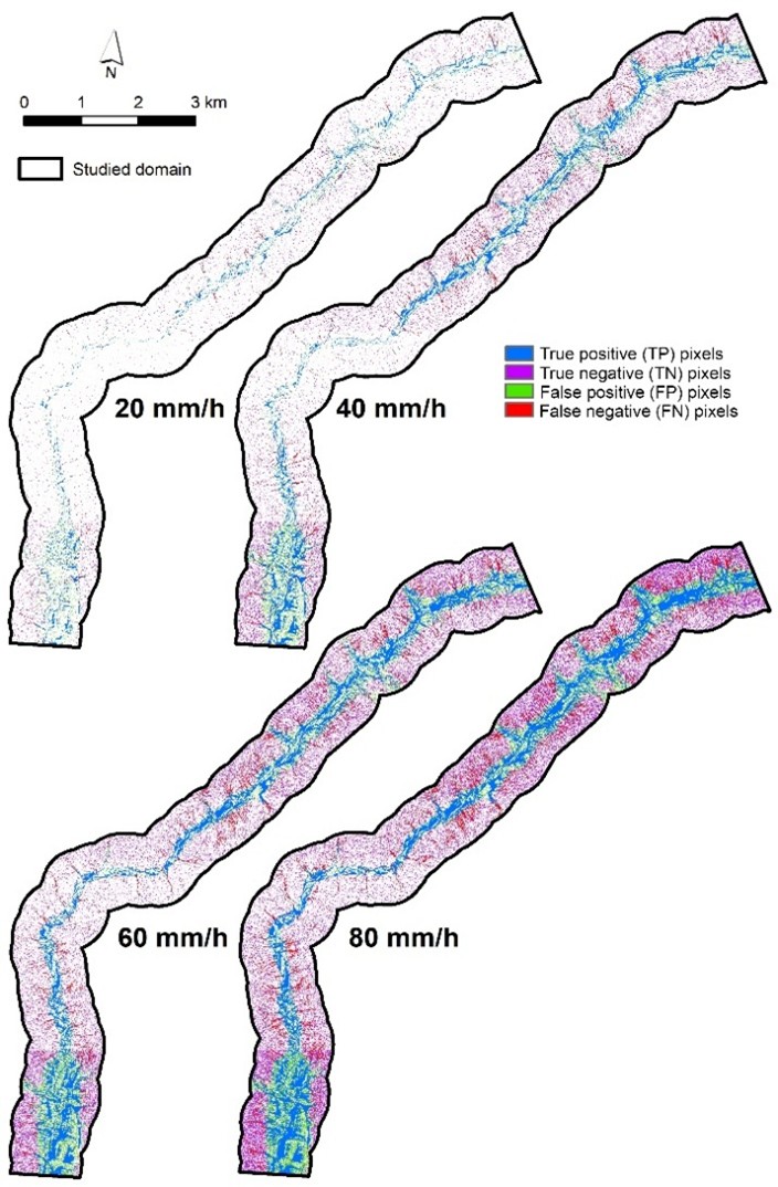
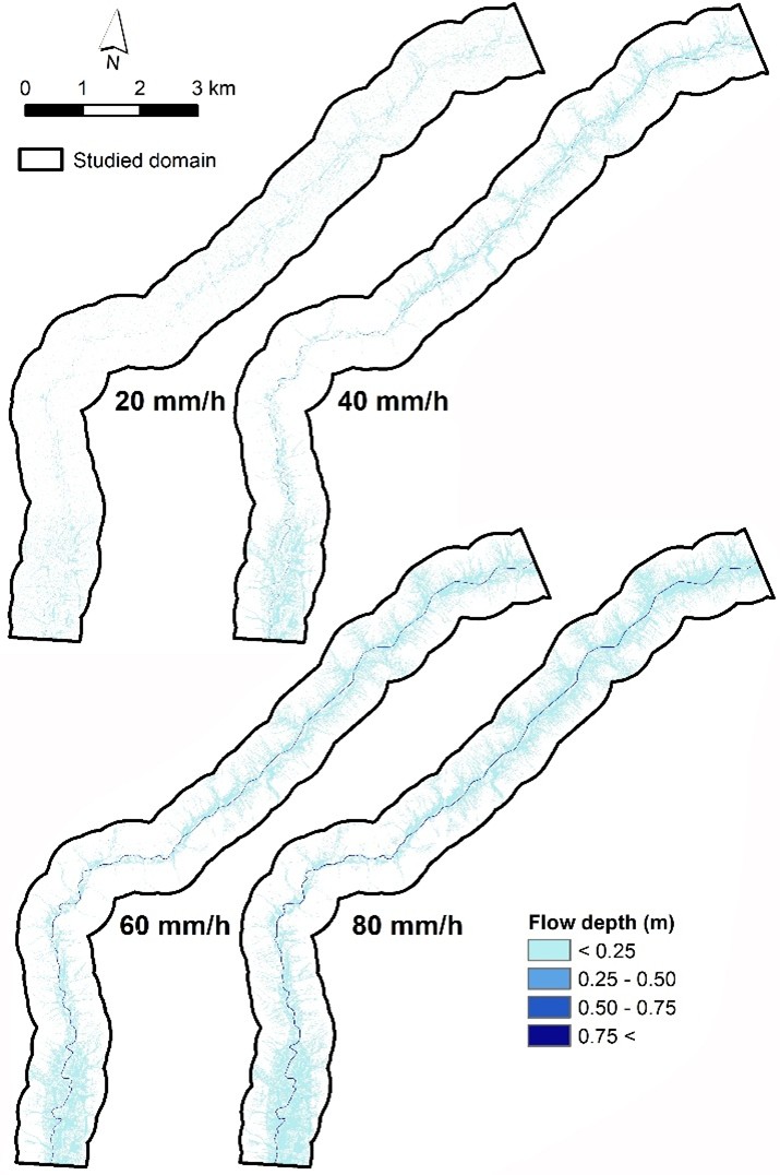
Based on the resulting XGB-ML models, four pluvial flood inundation maps were created for the Teplica domain. Figure 6 shows the pluvial flood extent classification maps for the studied rainfall scenarios. Figure 7 shows the resulting maps for water depth prediction performed by the XGB model. These maps were assembled from the held-out predictions of the ten spatial cross-validation runs: for each fold, predictions were generated by the model trained without that fold, and the fold-level predictions were then mosaicked to obtain the final domain-wide maps. The maps therefore represent cross-validated out-of-sample predictions rather than predictions from a single fold, an ensemble, or a final model fitted to all pixels.

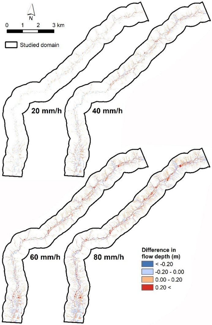
Difference in flow depths between the hydraulic and the XGB models for the studied rainfall scenario is shown in Figure 8. The biggest differences mainly concern the channel itself, local water bodies or deeper depressions (values higher than +-0.2 m). Most of the pixels belong to the intervals -0.2 – 0.0 m (from 45 to 49%) and 0.0 – 0.2 m (from 47 to 48%) in case of all studied rainfall scenarios.

3.5. Performance metrics of XGB model

Table 2 summarizes the performance of the XGB models for pluvial flood extent classification. Overall, the F1-score varies between 0.69 and 0.88, with improved model performance under lower intensity events (20 and 40 mm/h) relative to higher intensities (60 and 80 mm/h). The F1-score mean ± std summary statistics were 82.1 ± 4.4%, 79.8 ± 3.4%, 76.3 ± 2.4%, and 73.3 ± 2.9% for the rainfall scenarios of 20, 40, 60, and 80 mm/h, respectively. Spatially, models with lower intensity events tend to achieve higher F1-scores in upstream and central test folds while in case of models with higher intensity events, it is rather downstream folds which had better performance. In terms of computational efficiency, training times of XGB classification models ranged from 128.16 to 413.77 seconds, also due to larger domain extent. Classification inference on the held-out test folds was also rapid, with testing times ranging from 0.51 to 4.21 seconds. Expressed per tested pixel, this corresponds to an overall average inference time of approximately 1.37 µs/pixel.

The results of the regression analysis for pluvial flow depth prediction are presented in Table 3. The RMSE values ranged between 2.5% and 13.7% across the different rainfall scenarios. MAE recorded the range of values between 1.2 and 4.8%. Bias values indicate both overestimation and underestimation of hydraulically simulated water depths, ranging from −3.1% to 2.4%. These percentage-based errors refer to the scenario-specific normalized depth range described in Section 2.6. Interestingly, the largest RMSE and MAE values occur under lower rainfall intensities (20 and 40 mm/h), whereas higher intensity scenarios (60 and 80 mm/h) tend to produce more accurate predictions of water depths. The RMSE mean ± std summary statistics were 5.8 ± 2.8%, 4.1 ± 1.0%, 3.6 ± 0.7%, and 3.7 ± 0.8% and for the rainfall scenarios of 20, 40, 60, and 80 mm/h, respectively. The MAE mean ± std summary statistics were 2.6 ± 0.9%, 1.9 ± 0.5%, 1.6 ± 0.3%, and 1.6 ± 0.4% for the rainfall scenarios of 20, 40, 60, and 80 mm/h, respectively. The Bias mean ± std summary statistics were 0.2 ± 1.3%, 0.2 ± 0.6%, 0.0 ± 0.3%, and -0.0 ± 0.4% for the rainfall scenarios of 20, 40, 60, and 80 mm/h, respectively. Regarding the computational performance, XGB models demonstrate the training times ranging from 105.23 to 483.43 seconds. Regression inference on the held-out test folds ranged from 0.16 to 2.95 seconds, corresponding to an overall average inference time of approximately 0.74 µs/pixel. Despite the extent of the studied domain, these training and inference times remain acceptable for rapid pluvial flood inundation mapping.

Table 4 presents summary statistics for the test folds based on the F1-score, RMSE, MAE, and Bias metrics. Regarding the F1-score metric, the folds 5 and 6 (83.6 ± 3.2%) resulted in the highest mean values while the lowest SD was recorded in case of folds 8 and 2. The lowest mean values of F1-score were recorded for folds 2 and 3 and downstream folds 7, 8, and 9 while the highest SD was in case of folds 6 and 7. The highest mean values of RMSE and MAE metrics were in case of folds 0 and 5 while the lowest mean values were in case of folds 9 and 3. As for the Bias, the lowest mean and SD values were recorded for folds 3, 2, and 9.

3.6. Importance of predictors

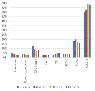
The relative mean importance of predictors for the XGB models in the classification task is presented in Figure 9. Across all rainfall scenarios and test folds, HAND consistently emerged as the most influential predictor, with mean importance values ranging from 50% to 59%. Slope ranked as the second most important predictor, with mean values between 16% and 20%. Roughness was identified as the third most relevant predictor, with mean importance values between 7% and 13%. The remaining predictors exhibited comparatively low contributions each below 6%.

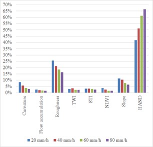
For the regression task using the XGB model, HAND again dominated as the most significant predictor, with markedly higher mean importance values ranging from 42% to 67% (Figure 10). Surface roughness ranked second, with mean values between 16% and 26%, while slope followed with mean importance ranging from 6% to 11%. All other predictors showed limited influence, with mean importance values remaining below 10%.

3.7. Limitations

In this sub-section, we acknowledge several limitations, which arise from the data or methodical steps used. First, the ML models were trained exclusively on hydraulically simulated flood data. Although hydraulic simulations provide extensive and internally consistent datasets suitable for ML training, the resulting emulations inevitably inherit the assumptions, simplifications, and uncertainties associated with the underlying hydraulic model. Consequently, the lack of validation against observed flood events limits the ability to assess model performance under real-world conditions and reduces confidence in the direct operational applicability of the proposed framework. Nevertheless, the primary objective of this study was not to evaluate the real-case accuracy of the hydraulic model itself, but rather to investigate how effectively ML models can reproduce flood extent and flow depth patterns derived from hydraulic simulations. In this context, the hydraulic model served mainly as a reference generator for the ML training process. Future research should therefore incorporate validation using observed flood extents and water-depth measurements once such datasets become available. This would enable a more rigorous assessment of the generalization capability, robustness, and practical applicability of the proposed ML framework under actual flood conditions.

A second limitation relates to the rainfall scenarios considered in the study. Only four rainfall scenarios with constant rainfall intensities were analyzed, while temporal variability in rainfall distribution was not incorporated. However, the selected rainfall intensities represent realistic precipitation magnitudes with plausible occurrence probabilities during 30-minute rainfall events within the study domain. Specifically, these intensities were chosen to reflect short-duration, high-intensity convective storms that are commonly associated with pluvial flooding processes. The lower-intensity scenarios (20 and 40 mm/h) correspond to moderate and relatively frequent pluvial rainfall events, whereas the higher-intensity scenarios (60 and 80 mm/h) represent more severe and extreme precipitation conditions capable of producing extensive surface runoff and widespread inundation. Employing multiple rainfall intensities also enabled an evaluation of ML model performance under varying levels of flood severity and hydraulic complexity. Constant rainfall intensities were intentionally adopted to isolate the influence of rainfall magnitude on both hydraulic simulations and subsequent ML emulation performance. This simplified experimental design facilitated a controlled comparison among rainfall scenarios while minimizing additional variability introduced by temporally heterogeneous rainfall patterns. Moreover, the selected rainfall intensities generated sufficiently distinct inundation responses, allowing the construction of diverse hydraulic training datasets across the investigated scenarios.

Finally, the transferability of the developed ML models was not evaluated beyond the investigated study area. Since the framework was trained and tested under specific topographic, hydrologic, and rainfall conditions, its applicability to other domains, climatic regions, or urban/peri-urban environments remains uncertain. Future work should therefore focus on evaluation of cross-domain transferability to improve the robustness of the proposed framework.

4. CONCLUSIONS

This study demonstrated the applicability of ML, specifically the XGB algorithm, for rapid pluvial flood inundation mapping using hydraulically derived training data and high-resolution spatial predictors in the Teplica domain. The hydraulic simulations by the MIKE+ model provided a basis for training and testing the ML models under multiple constant rainfall scenarios (20 - 80 mm/h), ensuring physically consistent representation of flood processes.

The multicollinearity analysis confirmed that all selected predictors were sufficiently independent, with Pearson correlation coefficients and VIF values well below the critical thresholds. This indicates that the predictor set was appropriate for ML modeling and did not introduce redundancy that could have negatively affected the model performance. The spatial analysis of predictors revealed moderate terrain gradients, relatively low STI values, and balanced moisture conditions, which together characterize the hydrological behavior of the Teplica domain. These factors, combined with land cover-based roughness and vegetation indicators, provided a comprehensive representation of flood-driving processes.

The XGB model achieved acceptable performance in both classification and regression tasks. For flood extent prediction, F1-scores ranged from 0.69 to 0.88, with better performance generally observed under lower rainfall intensities. In contrast, water depth prediction showed improved accuracy for higher rainfall scenarios, with RMSE values between 2.5% and 13.7% and low bias values. Spatial variability in performance was also observed, suggesting that model accuracy is influenced by both the rainfall intensity and the position of the test fold. From a computational perspective, the training and inference times remained within acceptable limits, even for a relatively large study domain. Inference was faster, remaining below 4.21 seconds for flood extent classification and below 2.95 seconds for water depth regression on the held-out test folds, corresponding to approximately 1.37 and 0.74 µs/pixel, respectively. This highlights the efficiency of the proposed approach and its suitability for rapid flood mapping. The analysis of predictor importance revealed that HAND is the dominant factor controlling both flood extent and depth, followed by slope and surface roughness. This emphasizes the critical role of topographic position relative to the drainage network in pluvial flood processes, while also confirming the relevance of terrain and land surface characteristics.

Overall, the results demonstrate that ML models trained on hydraulically derived data can effectively emulate flood inundation patterns with acceptable accuracy and significantly reduced computational cost, as the simulation time of hydraulic models was 1,458, 2,847, 4,151, and 6,130 seconds for the 20, 40, 60, and 80 mm/h rainfall scenarios, respectively. The proposed approach represents a promising tool for rapid pluvial flood hazard assessment and flood risk management in Slovakia and similar regions. After proper calibration/validation of the hydraulically derived maps used for ML training, the subsequent surrogate modeling results could be useful mainly for water and emergency managers, urban planners or insurance companies. Future research should focus on incorporating additional dynamic inputs, such as spatially variable rainfall or other high-resolution predictors, as well as testing the transferability of the ML models to other areas.

Funding

Funded by the EU NextGenerationEU through the Recovery and Resilience Plan for Slovakia under the project No. 09I03-03-V03-00085.

REFERENCES

• Alin, A., 2010. Multicollinearity. Wiley Interdisciplinary Reviews: Computational Statistics, 2(3), 370-374.
• Asif, M., Kuglitsch, M.M., Pelivan, I. & Albano, R., 2025. Review and Intercomparison of Machine Learning Applications for Short-term Flood Forecasting. Water Resources Management, 39, 1971–1991. https://doi.org/10.1007/s11269-025-04093-x
• Bartlett, M.S., Blitterswyk, J.V., Farella, M., Li, J., Smith, C., Parolari, A.J., Krishnamoorthy, L. & Mrad, A., 2025. Physically Based Dimensionless Features for Pluvial Flood Mapping with Machine Learning. Water Resources Research, 61(4), e2024WR039086. https://doi.org/10.1029/2024WR039086
• Bates, P.D., Quinn, N., Sampson, C., Smith, A., Wing, O., Sosa, J., Savage, J., Olcese, G., Neal, J., Schumann, G. & Giustarini, L., 2021. Combined modeling of US fluvial, pluvial, and coastal flood hazard under current and future climates. Water Resources Research, 57(2), e2020WR028673. https://doi.org/10.1029/2020WR028673
• Bentivoglio, R., Isufi, E., Jonkman, S.N. & Taormina, R., 2022. Deep learning methods for flood mapping: a review of existing applications and future research directions. Hydrology and Earth System Sciences, 26, 4345–4378. https://doi.org/10.5194/hess-26-4345-2022
• Berkhahn, S., Fuchs, L. & Neuweiler, I., 2019. An ensemble neural network model for real-time prediction of urban floods. Journal of Hydrology, 575, 743–754. https://doi.org/10.1016/j.jhydrol.2019.05.066
• Cea, L., Sañudo, E., Montalvo, C., Farfán, J., Puertas, J. & Tamagnone, P., 2025. Recent advances and future challenges in urban pluvial flood modelling. Urban Water Journal, 22(2), 149–173. https://doi.org/10.1080/1573062X.2024.2446528
• Chen, T. & Guestrin, C., 2016. XGBoost: A scalable tree boosting system. In Proceedings of the 22nd ACM SIGKDD International Conference on Knowledge Discovery and Data Mining, pp. 785–794.
• Chow, V.T., 1959. Open-Channel Hydraulics. McGraw-Hill Higher Education, New York. 
• Chu, H., Wu, W., Wang, Q., Nathan, R. & Wei, J., 2020. An ANN-based emulation modelling framework for flood inundation modelling: Application, challenges and future directions. Environmental Modelling & Software, 124, 104587. https://doi.org/10.1016/j.envsoft.2019.104587 
• Copernicus, 2024. Severe Flooding in Central and Eastern Europe. https://eu-space.europa.eu/components/earth-observation-copernicus/image-of-day/severe-flooding-central-and-eastern-europe, Accessed 13 February 2026.
• El Baida, M., Boushaba, F., Chourak, M. & Hosni, M., 2024. Real-Time Urban Flood Depth Mapping: Convolutional Neural Networks for Pluvial and Fluvial Flood Emulation. Water Resources Management, 38, 4763–4782. https://doi.org/ 10.1007/s11269-024-03886-w
• Guo, Z., Leitao, J.P., Simões, N.R. & Moosavi, V., 2021. Data-driven flood emulation: Speeding up urban flood predictions by deep convolutional neural networks. Journal of Flood Risk Management, 14, e12684. https://doi.org/10.1111/jfr3.12684
• Li, J., Pan, G., Chen, Y., Wang, X., Huang, P., Zhang, L. & Zhou, H., 2025. Rapid-Mapping Maximum Water Depth Map of Urban Flood Using a Highly Adaptable Machine Learning Based Model. Journal of Flood Risk Management, 18(3), e70095. https://doi.org/10.1111/jfr3.70095
• Liao, Y., Wang, Z., Chen, X. & Lai, C., 2023. Fast simulation and prediction of urban pluvial floods using a deep convolutional neural network model. Journal of Hydrology, 624, 129945. https://doi.org/10.1016/j.jhydrol.2023.129945
• Mediero, L., Soriano, E., Oria, P., Bagli, S., Castellarin, A., Garrote, L. Mazzoli, P., Mysiak, J., Pasetti, S., Persiano, S., Santillán, D. & Schröter, K., 2022. Pluvial flooding: High-resolution stochastic hazard mapping in urban areas by using fast-processing DEM-based algorithms. Journal of Hydrology, 608, 127649. https://doi.org/10.1016/ j.jhydrol.2022.127649
• Mudashiru, R.B., Sabtu, N., Abustan, I. & Balogun, W., 2021. Flood hazard mapping methods: A review. Journal of Hydrology, 603, 126846. https://doi.org/10.1016/j.jhydrol.2021.126846
• Pakdehi, M., Ahmadisharaf, E., Nazari, B. & Cho, E., 2024. Transferability of machine-learning-based modeling frameworks across flood events for hindcasting maximum river water depths in coastal watersheds. Natural Hazards and Earth System Sciences, 24, 3537–3559. https://doi.org/10.5194/nhess-24-3537-2024
• Rahmati, et al., 2018. Development and analysis of the Soil Water Infiltration Global database. Earth System Science Data, 10(3), 1237–1263. https://doi.org/10.5194/essd-10-1237-2018
• Rosenzweig, B.R., McPhillips, L., Chang, H., Cheng, C., Welty, C., Matsler, M., Iwaniec, D. & Davidson, C.I., 2018. Pluvial flood risk and opportunities for resilience. WIREs Water, 5(6), e1302. https://doi.org/10.1002/wat2.1302
• Rözer, V., Peche, A., Berkhahn, S., Feng, Y., Fuchs, L., Graf, T., Haberlandt, U., Kreibich, H., Sämann, R., Sester, M., Shehu, B., Wahl, J. & Neuweiler, I., 2021. Impact-based forecasting for pluvial floods. Earth's Future, 9, e2020EF001851. https://doi.org/10.1029/2020EF001851
• Sañudo, E., Gabrcía-Feal, O., Hagen, L., Cea, L., Puertas, J., Montalvo, C., Alvarado-Vicencio, R. & Hofmann, J., 2025. IberSWMM+: A high-performance computing solver for 2D-1D pluvial flood modelling in urban environments. Journal of Hydrology, 651, 132603. https://doi.org/10.1016/j.jhydrol.2024.132603
• Sejinja, I.W., Owor, N.J. & Mugume, S.N., 2025. A deep learning approach for urban pluvial flood depth estimation using citizen-generated data and physics-based validation. Journal of Hydroinformatics, 27(12), 1893–1917. https://doi.org/10.2166/hydro.2025.107
• Shao, Y., Chen, J., Zhang, T., Yu, T. & Chu, S., 2024. Advancing rapid urban flood prediction: a spatiotemporal deep learning approach with uneven rainfall and attention mechanism. Journal of Hydroinformatics, 26(6), 1409. https://doi.org/10.2166/hydro.2024.024
• Tamura, R., Kobayashi, K., Takano, Y., Miyashiro, R., Nakata, K. & Matsui, T., 2019. Mixed integer quadratic optimization formulations for eliminating multicollinearity based on variance inflation factor. Journal of Global Optimization, 73(2), 431–446. https://doi.org/10.1007/s10898-018-0713-3
• Teng, J., Jakeman, A.J., Vaze, J., Croke, B.F., Dutta, D. & Kim, S.J.E.M., 2017. Flood inundation modelling: A review of methods, recent advances and uncertainty analysis. Environmental Modelling & Software, 90, 201–216. https://doi.org/10.1016/ j.envsoft.2017.01.006
• Vojtek, M., Držík, D., Kapusta, J. & Vojteková, J., 2026a. Transferability of machine/deep learning-based prediction of fluvial flood extent to distinct river sections in Slovakia based on benchmark flood maps and high-resolution spatial data. Journal of Hydrology: Regional Studies, 65, 103339. https://doi.org/10.1016/j.ejrh.2026.103339
• Vojtek, M., Hačková, P., Melišková, P., Borsíková, A., Jakabová, Z. & Vojteková, J., 2026b. Pluvial flood hazard assessment in the Nitra River Basin, Slovakia. Carpathian Journal of Earth and Environmental Sciences, 21(1), 141–154. https://doi.org/10.26471/cjees/2026/021/359
• Vojtek, M., Janizadeh, S. & Vojteková, J., 2023a. Riverine flood potential assessment using metaheuristic hybrid machine learning algorithms. Journal of Flood Risk Management, 16(3), e12905. https://doi.org/10.1111/jfr3.12905
• Vojtek, M., Moradi, S., De Luca D. L., Petroselli, A. & Vojteková, J., 2024. Fluvial and pluvial flood hazard map-ping: combining basin and municipal scale assessment. Geomatics, Natural Hazards and Risk, 15(1), 2432377. https://doi.org/10.1080/ 19475705.2024.2432377
• Vojtek, M., Moradi, S., Petroselli, A. & Vojteková, J., 2025. Comparative analysis of hydraulic and GIS-based Height Above the Nearest Drainage model for fluvial flood hazard mapping: a case of the Gidra River, Slovakia. Stochastic Environmental Research and Risk Assessment, 39, 2657–2675. https://doi.org/10.1007/s00477-025-02988-0
• Vojtek, M. & Vojteková, J., 2026. Fluvial Flood Inundation Modeling: a Comparative Assessment of 1D and 2D Hydraulic Approach Using MIKE+. Water Resources Management, 40, 24. https://doi.org/10.1007/s11269-025-04423-z
• Vojtek, M., Vojteková, J., De Luca, D.L. & Petroselli, A., 2023b. Combined basin-scale and decentralized flood risk assessment: a methodological approach for preliminary flood risk assessment. Hydrological Sciences Journal. 63(3), 355–378. https://doi.org/10.1080/02626667.2022.2157279