1. INTRODUCTION

The river system is one of the most effective agents responsible for sediment redistribution through specific erosion, transport, and deposition processes (Mukteshwar, 2019). Fluvial modelling, in turn, is strongly sensitive to tectonic and lithological controlling factors (Ghosh, 2023). Fluvial incision can be approached based on longitudinal river profiles. This is a plot constructed on the basis of elevation and river channel length, from the headwater to the stream mouth (Antón et al., 2014). The analysis of longitudinal profiles can provide valuable information on how geological factors have influenced the fluvial processes responsible for the current appearance of the valleys, thus creating a history of the geomorphological evolution of the area (Kirby et al., 2003; Rădoane et al., 2003). Longitudinal river profiles are considered to be the result of the interaction between fluvial incision, lithology, tectonics, and base level change (Snyder et al., 2000; Duvall et al., 2004). All these controlling factors can lead to local distortions of longitudinal profiles, known as knickpoints and knickzones. A knickpoint is referred to as a slope break in a channel or a change in bed elevation. Knickpoints develop when crossing a hard lithology, a tectonic line, an injection site of coarse sediments, at tributary junctions (Ambili & Narayana, 2014; Bowman, 2023). A knickzone is a local segment, usually up to several kilometres long, with a higher gradient, sandwiched between lower gradient segments (Hayakawa & Oguchi, 2009). Knickpoints and knickzones provide valuable information regarding the lithological control, active erosion mechanism, tectonic uplift, and sea level change due to palaeoclimatic variation (Das, 2018). 

Among the variables that characterise the longitudinal profiles of rivers, the one that takes into account the variations in channel gradients seems to be the most commonly used. In this sense, the method for analyzing longitudinal profiles developed by Hack (1973), called Stream Length Gradient Index or SL Index (or Hack Index), proposes a quantitative parameter in numerical form, which can indicate whether a river is in equilibrium to its geomorphological context (Monteiro & Corrêa, 2020). This index represents the available stream power at a given point along a river bed (Pérez-Peña et al., 2009). Along the river the SL index can register different values, which can be mainly attributed to: (i) erosion resistant lithology; (ii) presence of coarse sediment deposits in the river channel; (iii) active tectonics; (iv) changes in the base level; (v) confluence with tributaries; (vi) anthropogenic activities; (vii) mass movements affecting the river bed (Seeber & Gornitz, 1983; El Hamdouni et al., 2010; Martinez et al., 2011; Troiani et al., 2014). It has been shown that there is a very good correlation between SL index values and the degree of erosion resistance of the rocks in which the river has deepened (Troiani & Della Seta, 2008). Thus, it has been observed that higher SL index values coincide with erosion-resistant rock areas or with bed sections with large-sized sediments, which effectively protect the river bed against fluvial erosion (Alipoor et al. 2011; Rădoane et al., 2017). The high SL index values recorded in areas with low erosion-resistant lithologies may be an indicator of active tectonics (Keller, 1986; Mishra, 2019). The high SL index values correspond to those sharp changes in the channel bed slope previously described and called knickpoints.

The Hack's SL index and other related indices have been quite often used to detect and explain various disturbances present along the longitudinal profiles of rivers: Seeber & Gornitz, 1983; Chen et al., 2006; Goldrick & Bishop, 2007; Troiani & Della Seta, 2008; Font et al., 2010; Troiani et al., 2014; Pérez-Peña et al., 2009; Troiani et al., 2017; Viveen et al., 2021; Roy et al., 2025.

In Romania, so far, there are only two papers that have strictly addressed the issue of longitudinal profile anomalies by means of the SL index, namely Rădoane et al., 2017; Cruceru et al., 2025. The former analysed the longitudinal profiles of some important rivers in the Eastern and South-Eastern Carpathians and the latter analysed the profiles of some rivers in the sector Iron Gates of the Danube.

The present study focused on analysing the steepness of the main stream channels in the Trotuș River basin, in relation to the structure and lithology of the deposits cut by the hydrographic network. The main objectives were: (i) to quantify the SL index and other correlated indices associated with the longitudinal profiles of the Trotuș and other 114 tributaries; (ii) to represent the spatial variability of the SL index and correlated indices (SL/K, for example) characteristic of the analysed profiles; (iii) to establish classes and threshold values for defining outliers for a given river; (iv) to locate and characterise the main knickpoints and knickzones in lithological and structural context.

2. STUDY AREA

The Trotuș River basin is located in the east-central part of the Eastern Carpathians (Figure 1). The Trotuș fault, over which part of this basin overlaps, is an important transition zone, in terms of the behaviour of rivers North and South of it (Rădoane et al., 2003; 2017).

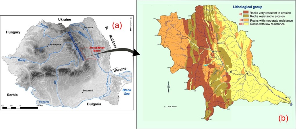
The substratum on which the Trotuș River basin is grafted belongs to four distinct structural and lithological units: the marginal syncline, the Carpathian flysch, the peri-Carpathian molasse and the foredeep (s.str.) zone. More than 57% of the total area (4350 km2), located in the upper and middle basin, is underlain by rocks belonging to the Carpathian Flysch (sandstones, conglomerates, marls, and clays). The East-Carpathian Flysch comprises five nappes named, from west to east, as follows: Ceahlău, Teleajen, Audia, Tarcău and Vrancei; 23.3% of the surface area belongs to the pericarpathic molasse domain, characteristic of the middle basin-lower basin transition zone (marls, clays, sands, sandstones); on 17.5% of the surface area occur Quaternary deposits, with the largest extension in the lower course (gravels, sands, loess deposits); 1.7% of the surface area belongs to the crystalline-Mesozoic zone, located in the upper course, characterised by the presence of crystalline schists, intrusive rocks, limestones and conglomerates (Dumitriu, 2014; 2020).

Based on the information on rock hardness, relative relief and the gradient of longitudinal profiles (Dumitriu 2014) separated three lithological groups with different erosion resistance, namely (Figure 1):

(i) a lithological group with high resistance to erosion (comprises the areas with resistant and very resistant rocks to erosion in Figure 1), it extends over about 1680 km2 (about 38% of the basin area) and overlaps the western and central part of the Carpathian Flysch area, holding the largest area within the mountain basins of the Oituz, Slănic, Dofteana, Uz, Ciobănuș and Asău rivers; (ii) a lithological group with moderate resistance to erosion - covers about 22% of the entire basin area and is characteristic of the upper Trotuș River basin, upstream of the confluence with the Sulța river; (iii) a lithological group with low resistance to erosion (about 40% of the basin area), occupies the entire area of the Quaternary deposits and most of the Molasse, except for a few small areas where a series of more resistant deposits occur.

3. MATERIALS AND METHODS

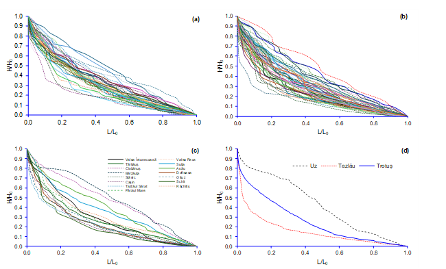
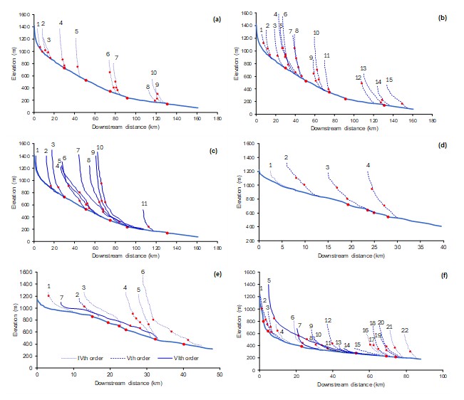
The necessary data (elevation and length of the river at a given point) for the longitudinal profiles were extracted from 1:25000 topographic maps. In order to be comparable, the real longitudinal profiles were reduced to unity in order to obtain a dimensionless size (as H/Ho - L/Lo - ratio of altitude - ratio of distance), capable of eliminating possible errors introduced by the differences in scale of river length in relation to altitude (Rădoane et al, 2003). 115 longitudinal profiles were constructed and analysed with the extracted data (40 profiles of IVrd order rivers in the Strahler system; 57 of Vth order rivers; 15 of VIth order rivers; 2 of VIIth order and 1 of VIIIth order - Trotuș). The choice of these longitudinal profiles for analysis was made considering the length of the rivers, the surface of the basins, the structural and lithological complexity of the drainage basins, etc.

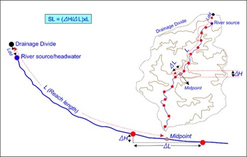
The SL index (Stream-Length gradient index), which indicates deviations from an equilibrium or "ideal" longitudinal profile caused by tectonic, lithological, climatic or anthropogenic factors, was calculated using the formula proposed by Hack (1973) (Figure 2): 

where ΔH and ΔL are the difference in height and length between two points and L is the total length, measured from the divide (or from the river source) to middle of that two points.

Low values of SL index may reflect either an area with active tectonic subsidence (Viveen et al., 2012) or the presence of rocks with low erosion resistance (Žibret & Žibret, 2014). High values of SL index may indicate either an area with strong tectonic uplift or the sectioning of erosion-resistant rocks (Alipoor et al., 2011). Theoretically, in a lithologically homogeneous catchment, the SL index will be approximately constant (Antón et al., 2014).

The SL/K index (where SL represents the Hack index and K represents the index in the semi-logarithmic form) proposed by Seeber and Gornitz (1983), who adapted the methodology initially put forward by Hack (1973) to understand the equilibrium relationship between landform elements based on the analysis of drainages and their longitudinal profiles (Monteiro & Corrêa, 2020), was also calculated:

where i and j refer to two points along the drainage profile and lnL is the natural logarithm of L. In this study the K index was calculated for the entire longitudinal profile, in which case equation (3) was used:

where lnL is the natural logarithm of the length of the longitudinal profile between the source and the confluence. In this case K index is also called SLtotal index. The SL/SLtotal ratio was calculated, where the SL index values of each section were divided by the K index value calculated for the entire longitudinal profile. Ghosh (2023) calls this index the Normalised Stream-Length gradient index (NSL). When the values of this ratio are less than 2 (SL/K < 2), the section would be close to the ideal profile expected for the elevation difference and the channel length. When the ratio is greater than or equal to 2 (SL/K ≥ 2), the sector is considered steep or abrupt. When the value is higher than 10 (SL/K ≥ 10), the sector is considered very steep or very abrupt (Seeber & Gornitz, 1983). For sectors with values equal to or greater than 2, applying a similar methodology, Etchebehere et al. (2006) and Martinez et al. (2011) attributed the term "anomalous", being the stretches with values between 2 and 10 classified as second order anomalies and segments with values equal to or above 10 as first order anomalies (Monteiro & Corrêa, 2020).

The slope gradient index (S) describes the change in SL index between chosen segments and shows where the highest rates of SL changes are located. This index can be calculated using the following equation (4):

where Δslope is the difference in slope between two adjacent segments. ΔL is the mid-point between the lengths of two segments, L is the length of the channel from the point of interest where the slope gradient index is calculated to the source of the channel. The dimensionless values of S can be positive or negative. Positive values indicate change from a steep to a less steep segment, and negative values indicate an increase in segment steepness for a constant gradient S = 0 (Ambili & Narayana, 2014).

An issue often discussed in the literature is the threshold values of the SL index above which one can talk about those longitudinal profile anomalies called knickpoints. The threshold values differ from author to author and these were considered the SL index values lying above: the mean value of the SL index; the standard deviation value (+1SD) (Das, 2018).

In this paper, SL values higher than the mean on a basin-by-basin basis were considered as anomalies. As presented by Aringoli et al. (2014) the anomalies of each longitudinal profile were divided into three different classes according to the standard deviation of the SL index values. The first class includes the values comprised between the average SL and one standard deviation values (1SD); the second class, SL values comprised between one standard deviation and two standard deviation values (2SD); the third class includes values greater than two standard deviations. Regarding the first class, it was observed that in some situations the average SL index values are greater than SD, so in these cases there will be only two classes, namely: one comprised between 1SD and 2SD, and the second one that includes values greater than 2SD. By using the same data (mean and standard deviation of SL index values) for classification, the method proposed by Das (2018) seems to have more conclusive results.

In many papers, the classification of SL index values has been based on the classes proposed by El Hamdouni et al. (2008), classes that reflect the degree of tectonic activity or the erosion resistance of rocks. The three classes are: class 1 (SL≥500), class 2 (300≤SL<500), and class 3 (SL<300).

4. RESULTS AND DISCUSSION

4.1. Longitudinal profiles  

The first step in analysing the SL index values is to produce longitudinal profiles of the rivers included in the study. A total of 115 longitudinal profiles were constructed for rivers from order IV to order VIII in Strahler system (Figure 3).

The intrinsic characteristic of a river bed is to evolve towards a longitudinal equilibrium profile, i.e. one with an equilibrium bed slope (an equilibrium bed slope) that allows the river to transport exactly the sediment load supplied from the upstream (Gao et al., 2020).

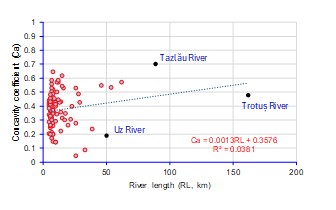
The shape of a river's longitudinal profile can provide a huge amount of information about the river's evolutionary stages. Among the parameters describing the shape of a longitudinal profile, the coefficient of concavity (Ca) seems to be the most important. This index was calculated (following the method presented by Rădoane et al., 2003) for all 115 longitudinal profiles analysed. The concavity coefficients ranged between: 0.625 (Frumoasa, in the Tazlău river basin) and 0.142 (Bașca, in the Uz river basin) for rivers of order IV; between 0.616 (Apa Lină, in the Uz river basin) and 0.140 (Ugra, tributary of the upper Trotuș River) for rivers of order V; between 0.584 (Schit, in the Tazlău catchment) and 0.044 (Bărzăuța, in the Uz catchment) for rivers of order VI; 0.700 - Tazlău and 0.190 - Uz for rivers of order VII. The longitudinal profile of the Trotuș River has a concavity coefficient of 0.480. According to Rădoane et al. (2003), the values of the concavity coefficient can be interpreted as follows: if its value is close to 0, the form of the profile is close to a straight line; if its value is close to 1.0, the profile is L-shaped.

Wheeler (1979) observed that there is a positive correlation between the concavity of longitudinal profiles and their length, and Leopold and Langbein (1962) showed that longitudinal profiles are straighter when their length is shorter. The rivers analysed in the present study, as in the examples presented by Larue (2011), do not show very strong correlations between the concavity coefficient of the longitudinal profiles and their length or gradient, probably because tectonic and lithological controlling factors were more strongly manifested (Figure 4). The significant role of these controlling factors is also confirmed by Gailleton et al. (2021). For rivers that dissect rocks with lower erosion resistance, the concavity of the longitudinal profiles is more pronounced (generally with values above 0.500) and the anomalies given the presence of high gradient sections quite small.

4.2. Stream-length gradient index (SL) -Trotuș River

In the case of the Trotuș River, the extreme values of the SL index ranged from 1150 (at the contact between the Flysch and the Molasse zone) to 50 (near the springs), with an average value of 342 (Figure 5a). Only in 19% of the analysed segments did the SL index values exceed the threshold of 500 (proposed by El Hamdouni et al., 2008), cases in which a strong involvement of tectonic and lithological factors is considered.

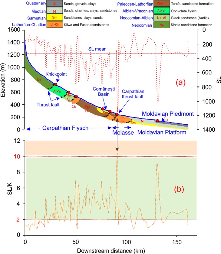
In general, the highest values of the SL index coincide with thrust faults located at the demarcation of the Carpathians flysch nappes or in the area of lithological contacts where rocks with high erosion resistance occur (Figure 5a). This situation has also been described for other rivers crossing mountainous areas (Harkins et al., 2005; Anand & Pradhan, 2019). The lower values of SL index seem to be associated with segments dominated by rocks with lower erosion resistance or characterised by low tectonic activity, which is consistent with the observations made by Hack (1973).

4.3. Stream-length gradient index (SL) - tributaries 

In the case of the IVth order tributaries, the highest SL index value (1850) was recorded for the longitudinal profile of the Bașca River in the Uz River basin. The segment where this value was recorded is located within the erosion-resistant rock area. The lowest value of SL index (24) belongs to a segment along the Gutinaș River, a tributary of the Trotuș in the lower course, where rocks with low erosion resistance predominate. The mean value of SL index values recorded for the fourth order rivers was 235. Only about 10% of the analysed segments had SL index values above 500, the threshold value for high-gradient sections (Figure 6a). 17% of the SL index values fell into class 2 (300≤SL<500) and the remaining 73% into class 3 (SL<300).

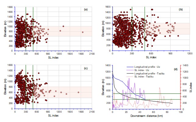
For Vth order rivers, a total of 1067 segments were analysed, of which about 8% fell into class 1 (SL≥500), 15% into class 2, and 77% into class 3. Of the values included in class 1, almost 60% were located in the middle and upper reaches basins at elevations between 600-1000 m. The mean SL index value for the 1067 segments was 220. The maximum value of SL index (1020) was recorded for a segment of the Șopan River (right tributary of the Trotuș River in the Comănești Depression) and corresponds to an insular area with erosion-resistant rocks (Figure 6b). The minimum value (8) belongs to a sector of the Orășa River (tributary of the Tazlău River), whose basin entirely overlaps the area of rocks with low erosion resistance.

For the VIth order rivers, out of the 724 segments analysed, 16% were in class 1 (67% of these values were in the middle and upper reaches at altitudes between 600-800 m), 23% in class 2, and 61% in class 3. The mean SL index value for this category of rivers was 300. The maximum value was 1730 and it was recorded in the lower course of the Ciobănuș river, in a sector with highly erosion-resistant rocks (Figure 6c). The minimum value (9) belongs to a sector in the upper reaches of the Răchitiș river in the Tazlău basin, which is grafted on weakly resistant rocks of the Carpathian Molasse.

In the case of the two VIIth order rivers, the maximum values are 974 for the Uz river (value recorded in the middle course at an altitude of 640 m) and 694 for the Tazlău river (in the lower course at an altitude of 230 m) (Figure 6d). The mean SL index values emphasise the tectono-structural characteristics of the two basins: 400 in the case of the Uz River and 192 in the case of the Tazlău River.

By analysing the geological maps, it was observed that the highest SL index values (generally above 500) recorded for the rivers analysed in this study correspond, as in very many other examples in the literature (Kale & Shejwalkar, 2008; Taloor et al., 2023; Roy et al., 2025), to sections with erosion-resistant rocks or active tectonic lines.

4.4. SL/K index

This index is used for a more accurate determination of anomalies along longitudinal profiles, called knickpoints/knickzones. It was found that first-order anomalies of this index (values greater than 10) have a very high rate of correspondence with the field realities (Monteiro & Corrêa, 2020).

The SL/K index is considered to be very sensitive to small deviations from the graded profile, which can be caused by different controlling factors, among which lithology plays an important role (Kirby & Whipple, 2012; Viveen et al., 2021). In the case of this index, in the first-order anomaly class (SL/K<10) we have many fewer values than in the first-order class of the SL index (SL≥500) (Figure 7). For example, for fourth-order rivers in class 1 of the SL index, we have 70 sectors, while in the SL/K<10 class, we have only 30 segments, but much more evident along the longitudinal profile. Another eloquent example is the Trotuș River, where class 1 of the SL index comprises 20 segments, and class 1 of the SL/K index only one sector, namely the one located at the contact of the Marginal Fold with the Pericarpathian Nappes. Along the longitudinal profile of the Uz River, the SL/K index shows 4 values above 10 (while the SL index had 18 values in class 1), all recorded in the middle course (3 at altitudes between 600-700 m and one at an altitude of about 500 m).

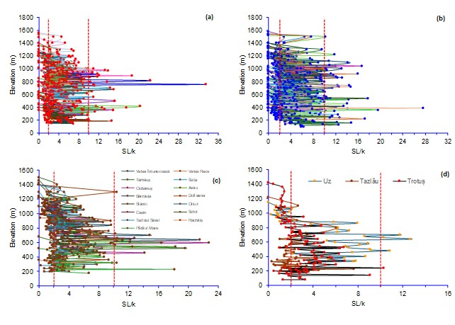
For all the 115 analysed rivers, the maximum value was 34 and was recorded for a segment along the Bașca River in the Uz river basin (described in SL index) (Figure 7a).

In most situations, the localisation within longitudinal profiles of SL/K index values greater than 10 confirms the conclusions presented in the literature that lithological and tectonic factors have the greatest influence in shaping these anomalies (Seeber & Gornitz, 1983; Colombo et al., 2000; Patel et al., 2022). However, not in all cases do these factors rank first in terms of the cause of anomalies along longitudinal profiles (Mishra, 2019; Das et al., 2025). In some studies, the mean value of SL/K, relative to the entire longitudinal profile, has also been considered (Gu et al., 2019). For example, the mean SL/K index values calculated for the rivers of order VII and VIII (Uz - 5.2, Tazlău - 2.1, and Trotuș - 3.1) accurately reflect the complexity of longitudinal profiles in terms of their anomalies (Figure 7d).

4.5. Classification of SL and SL/K index values

The interpretation of the results is also highly dependent on the categorisation of the obtained values into certain classes reflecting the influence of control factors. In this study, four classifications were used, namely: those proposed by El Hamdouni et al. (2008), Aringoli et al. (2014), and Das (2018) for SL index values; the classification proposed by Seeber & Gornitz (1983) with the additions made by Etchebehere et al. (2006) and Martinez et al. (2011) for SL/K index.

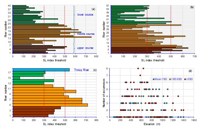
Another method used in this study to detect knickpoints and knickzones anomalies is the one proposed by Das (2018). That method proposes a threshold value of the SL index. The threshold was considered to be the result of the sum of the mean of the SL index values and their standard deviation (mean + 1 SD). Above this threshold value, all the sectors were considered as longitudinal profile anomalies. The highest values of this threshold were recorded in the middle course (Bașca - 754; Ciobănuș - 716; Uz - 664; Șugura - 645), where a mosaic of petrographic entities is delimited by thrust tectonic fault lines (Figure 8a,b,c).

By analysing the SL and SL/k index values according to lithological and structural conditions, it was found that the most evident anomalies of the longitudinal profiles are in class 1 of the classification presented by Seeber & Gornitz (1983) and above the threshold value given by mean+1SD. Under these conditions, the analysis of knickpoints and knickzones anomalies, lithologically and structurally, referred to SL and SL/K index values higher than these two thresholds. For the classification proposed by El Hamdouni et al. (2008), no obvious correlations with lithology or tectonics were found for all SL index anomalies included in class 2. Obvious lithological or structural explanations were found for all SL index anomalies with values greater than mean + 1SD. For this reason, this classification was chosen to discuss the nature of the anomalies along the longitudinal profiles. However, there were also a few anomalies, localised in areas of uniform, low erosion resistant lithology, which could not be fully explained.

By applying the classification method proposed by Aringoli et al. (2014), it was possible to rank the number of anomalies according to the altitudinal stages (Figure 8d). For example, for rivers of order VI, VII, and VIII, class 1 (>2SD) anomalies at altitudes of 540 and 640 m were recorded for 8 rivers (representing 45% of the rivers of these orders). These obvious anomalies are localised along the longitudinal profiles of the following rivers: Valea Întunecoasă (the anomaly at 540 m, located at the contact of the Hășmaș Syncline - with the Ceahlău Nappe; Asău (at 640 m, in the section area of a fold in the Tarcău Nappe); Bărzăuța (at 540 m, it presents the same situation as in the case of Asăului); Slănic (with anomalies both at 540 m and at 640 m, related to the lithostructural complications due to the presence of the Tarcău and Vrancei nappes); Cașin (at 540 m, an anomaly at the contact between the Vrancei nappe and the Pericarpathian molasse); Schit (tributary of the Tazlău, at 640 m, an anomaly arising from a similar situation to that of Cașin); Trotuș (at 640 m, closely related to the contact between the Audia and Tarcău nappes; at 540 m, an anomaly in the contact sector between the Tarcău and Vrancei nappes).

4.6. Knickpoint and knickzone anomalies

The anomalies with the highest values of SL and SL/K index, and which are well highlighted in the longitudinal profile of the studied rivers, were analysed in terms of possible relationships with lithology and tectonics. All these sectors of abrupt slope change in the longitudinal profiles, called knickpoints or knickzones, were localised on each profile (Figure 9).

Along the longitudinal profile of the Trotuș River, 7 more important knickpoint sectors have been identified (Figure 5 and 9 a,b,c): (i) at the altitude of 720 m, located at the contact between the Ceahlău and Teleajen nappes; (ii) at the altitude of 595 m, at the contact between the Teleajen and Audia nappes; (iii) at the altitude of 528 m, in the contact sector between the Audia and Tarcău nappes; (iv and v) at 460 and 440 m, at the entrance and exit of the Trotuș from the Comănești Depression, due to lithological changes; (vi) the most important, at 240 m altitude, in the transition sector between the Carpathian Flysch and molasse zones; (vii) at 140 m altitude, in the transition zone towards the pericarpathic piedmont (Rădoane & Rădoane, 2005).

In the case of the tributaries of the Trotuș River, the main knickpoint anomalies are located either at the contact of the main thrust nappes (Sulța, Ciobănuș, Uz, Slănic, Oituz, etc.), or in the contact sectors of lithological features with different erosion resistance (Tărhăuș, Ciugheș, Camenca, Agăș, Asău, etc.).

For a number of longitudinal profiles, a series of anomalies were observed at different altitudinal levels within a lithological group with similar erosion resistance. For example, in the case of the rivers Asău and Uz, in the sector where they cross the Tarcău Nappe. In this case, it is possible that, in addition to lithology, a series of structural elements (folds type anticline and syncline) are of particular importance in the occurrence of such anomalies.

As far as the Tazlău River is concerned, since its basin mostly overlaps the area of rocks with low erosion resistance and the number of notable anomalies is lower. The most important one is located at an elevation of about 230 m and also seems to be related to an anticlinal structural element. The second knickpoint is located in the Flysch area (at an elevation of 800 m) and seems to originate from a contact between two thrust nappes.

 It is difficult to determine the exact cause of these anomalies using solely geological maps, especially if they are located in sectors where a lithological contact and a fault thrust also occur. In these cases, we mainly attributed these anomalies to the lithological factor. The comparison of the results obtained with the field situation will be another stage of this study.

5. CONCLUSIONS

Analysing the anomalies along the longitudinal profiles of rivers is of particular importance in determining the main stages of evolution of the river network and the controlling factors that have influenced this evolution. These anomalies were quantified, localised and described on the basis of SL index values and other associated indices commonly used in studies of this kind. For this study, 115 longitudinal profiles (of the Trotuș River and 114 tributaries) were analysed. The first step of the analysis was to determine the spatial variability of the SL index and other associated indices. Among the associated SL indexes, the SL/K index was emphasised in this study, as it allows a more accurate determination of knickpoints/knickzones anomalies. 

The values obtained were categorised according to the criteria described in the literature. Some of these criteria were sometimes slightly adapted to the analysed situation. The highest values (usually placed in class 1 of these classifications) were considered as longitudinal profile anomalies and consequently analysed in terms of lithological and tectonic controlling factors.

Along the longitudinal profile of the Trotuș River, 7 knickpoint sectors were identified, all of them mainly due to the presence of lithological features with high erosion resistance. A number of these sectors are located on the path of thrust faults, so that it is rather difficult to separate the two controlling factors. The presence of the 5 thrust nappes, each containing rocks with different degrees of erosion resistance, seems to have favoured the occurrence of these anomalous sections along the longitudinal profiles of the analysed rivers.

Similarly, in the longitudinal profiles of the tributaries analysed, a correlation could be established between the location of most of the identified anomalies and the lithological and tectonic controlling factors. The presence of such anomalies in areas with low erosion-resistant rocks was more difficult to explain, but the cases were rather isolated.

REFERENCES

• Alipoor, R., Poorkermani, M., Zare, M., El Hamdouni, R., 2011. Active tectonic assessment around Rudbar Lorestan dam site, High Zagros Belt (SW of Iran). Geomorphology 128 (1–2), 1–14, https://doi.org/10.1016/j.geomorph.2010.10.014.
• Ambili, V., & Narayana, A. C., 2014. Tectonic effects on the longitudinal profiles of the Chaliyar River and its tributaries, southwest India. Geomorphology, 217, 37-47, https://doi.org/10.1016/j.geomorph.2014.04.013.
• Anand, A. K., & Pradhan, S.P., 2019. Assessment of active tectonics from geomorphic indices and morphometric parameters in part of Ganga basin. Journal of Mountain Science, 16(8), 1943-1961, https://doi.org/10.1007/s11629-018-5172-2.
• Antón, L., De Vicente, G., Muñoz-Martín, A., & Stokes, M., 2014. Using river long profiles and geomorphic indices to evaluate the geomorphological signature of continental scale drainage capture, Duero basin (NW Iberia). Geomorphology, 206, 250-261, https://doi.org/10.1016/j.geomorph.2013.09.02.
• Aringoli, D., Cavitolo, P., Farabollini, P., Galindo-Zaldivar, J., Gentili, B., Giano, S. I., ... & Troiani, F., 2014. Morphotectonic characterization of the Quaternary intermontane basins of the Umbria-Marche Apennines (Italy). Rendiconti Lincei, 25, 111-128, https://doi.org/10.1007/s12210-014-0330-0.
• Bowman, D., 2023. Discontinuity in Slope-Knickpoints and Knickzones. In: Base-level Impact. Springer, Cham. https://doi.org/10.1007/978-3-031-24994-5_3.
• Chen, Y.C., Sung, Q., Chen C.N., Jean, J.S., 2006. Variations in tectonic activities of the central and southwestern Foothills, Taiwan, inferred from river hack profiles. Terr. Atmos. Ocean. Sci., 17, 563-578, 10.3319/TAO.2006.17.3.563(T).
• Colombo, F., Busquets, P., Ramos, E., Vergés, J., & Ragona, D., 2000. Quaternary alluvial terraces in an active tectonic region: the San Juan River valley, Andean ranges, San Juan Province, Argentina. Journal of South American Earth Sciences, 13(7), 611-626, https://doi.org/10.1016/S0895-9811(00)00050-X.
• Cruceru, N., Rădoane, M., Perșoiu, I., Vespremeanu-Stroe, A., Ruszkiczay-Rüdiger Z., 2025. Tracing landscape evolution using stream profile analysis along the Iron Gates, Danube River, Romania. Geomorphology, 483, 109837, https://doi.org/10.1016/j.geomorph.2025.109837.
• Das, S., 2018. Geomorphic characteristics of a bedrock river inferred from drainage quantification, longitudinal profile, knickzone identification and concavity analysis: a DEM-based study. Arabian Journal of Geosciences, 11(21), 680, https://doi.org/10.1007/s12517-018-4039-8.
• Das, S., Roy, S., Chatterjee, J., Jaman J.M.H., Sengupta, S., 2025. Identifying topographic disequilibrium conditions and their lithological and tectonic implications in a rifted river basin of Eastern India: Insights from DEM-derived longitudinal profiles and their derivatives. J Earth Syst Sci., 134, 24, https://doi.org/10.1007/s12040-024-02492-z.
• Dumitriu, D., 2014. Source area lithological control on sediment delivery ratio in Trotus Drainage Basin (Eastern Carpathians). Geogr. Fis. Dinam. Qat., 37, 91–100, Doi 10.4461/GFDQ. 2014.37.08.
• Dumitriu, D., 2020. Sediment flux during flood events along the Trotuș River channel: hydrogeomorphological approach. J Soils Sediments, 20, 4083–4100, https://doi.org/10.1007/s11368-020-02763-4.
• Duvall, A., Kirby, E., Burbank, D., 2004. Tectonic and lithologic controls on bedrock channel profiles and processes in coastal California. J. Geophys. Res. 109, F03002, https://doi.org/10.1029/2003JF000086.
• El Hamdouni, R., Irigaray, C., Fernández, T., Chacón, J., Keller, E.A., 2008. Assessment of relative active tectonics, southwest border of the Sierra Nevada (southern Spain). Geomorphology 96, 150–173, https://doi.org/10.1016/j.geomorph.2007.08.004.
• El Hamdouni, R., Irigaray, C., Jiménez-Perálvarez, J.D., Chacón, J., 2010. Correlations analysis between landslides and stream length-gradient (SL) index in the southern slopesof Sierra Nevada (Granada, Spain). In: Williams, A.L., Pinches, G.M., Chin, C.Y., McMorran, T.J., Massey, C.Y. (Eds.), Geologically Active. Taylor and Francis Group, London, pp. 141–149.
• Etchebehere, M.L.C., Saad, A.R., Santoni, G., Casado, F.C., Fulfaro, V.J., 2006. Detecção de prováveis deformações neotectônicas no Vale do Rio do Peixe, Região Ocidental Paulista, mediante aplicaçao de Índices RDE (Relac̈ão Declividade-Extensão) em segmentos de drenagem. Geociências, 25(3), 271-289.
• Font, M., Amorese, D., & Lagarde, J.L., 2010. DEM and GIS analysis of the stream gradient index to evaluate effects of tectonics: the Normandy intraplate area (NW France). Geomorphology, 119(3-4), 172-180, https://doi.org/10.1016/j.geomorph.2010.03.017.
• Gailleton, B., Sinclair, H. D., Mudd, S. M., Graf, E. L., & Matenco, L. 2021. Isolating lithologic versus tectonic signals of river profiles to test orogenic models for the Eastern and Southeastern Carpathians. J. Geophys. Res. Earth Surf., 126, e2020JF005970, https://doi.org/10.1029/2020JF005970.
• Gao, W., Li, D., Wang, Z. B., Nardin, W., Shao, D., Sun, T., Miao, C., Cui, B., 2020. The longitudinal profile of a prograding river and its response to sea level rise. Geophysical Research Letters, 47(21), e2020GL090450, https://doi.org/10.1029/2020GL090450.
• Ghosh, B., 2023. Assessment of basin-scale geomorphic processes based on the analysis of longitudinal profiles: A case study of the Dwarkeswar river, Eastern India. Geology, Ecology, and Landscapes, 9(1), 317-333, https://doi.org/10.1080/24749508.2023.2202434.
• Goldrick, G., Bishop, P., 2007. Regional analysis of bedrock streamlong profiles: evaluation of Hack's SL form, and formulation and assessment of an alternative (the DS form). Earth Surf. Process. Landf., 32, 649–671, https://doi.org/10.1002/esp.1413.
• Gu, Z., Fan, H. & Song, Z., 2019. Quantitative analysis of the macro-geomorphic evolution of Buyuan Basin, China. Journal of Mountain Science,16, 1035–1047, https://doi.org/10.1007/s11629-018-5289-3.
• Hack, J.T., 1973. Stream-profiles analysis and stream-gradient index. J. Res. U.S Geol. Surv. 1, 421–429.
• Harkins, N.W., Anastasio, D.J., Pazzaglia, F.J., 2005. Tectonic geomorphology of the Red Rock fault, insights into segmentation and landscape evolution of a developing range front normal fault. Journal of Structural Geology, 27(11), 1925-1939, https://doi.org/10.1016/j.jsg.2005.07.005.
• Hayakawa, Y.S. & Oguchi, T., 2009. GIS analysis of fluvial knickzone distribution in Japanese mountain watersheds. Geomorphology, 111, 27-37, https://doi.org/10.1016/j.geomorph.2007.11.016.
• Kale, V.S., Shejwalkar, N., 2008. Uplift along the western margin of the Deccan Basalt Province: is there any geomorphometric evidence? Journal of Earth System Science, 117, 959–971, https://doi.org/10.1007/s12040-008-0081-3.
• Keller, E.A., 1986. Investigation of active tectonics: use of surficial Earth processes. In: Wallace, R.E. (Ed.), Active Tectonics. Studies in Geophysics. National Academy Press, Washington DC, pp. 136–147.
• Kirby, E., Whipple, K.X., Tang, W., Chen, Z., 2003. Distribution of active rock uplift along the eastern margin of the Tibetan Plateau; inferences from bedrock channel longitudinal profiles. J. Geophys. Res. 108 (4), 24, https://doi.org/10.1029/2001JB000861.
• Kirby, E., Whipple, K.X., 2012. Expression of active tectonics in erosional landscapes. J. Struct. Geol., 44, 54-75, https://doi.org/10.1016/j.jsg.2012.07.009.
• Larue, J.P., 2011. Longitudinal profiles and knickzones:the example of the rivers of the Cher basin in thenorthern French Massif Central. Proc.Geol.Assoc.122, 125–142, https://doi.org/10.1016/j.pgeola.2010.08.006.
• Leopold, L.B., Langbein, W.B., 1962. The concept of entropy in landscape evolution. United States Geological Survey Professional Paper 500 A, 3–20.
• Martinez, M., Hayakawa, E., Stevaux, J.C., Profeta, J.D., 2011. SL index as indicator of anomalies in the longitudinal profile of the Pirapó River. Rev. Geociências 30(1), 63–76.
• Mishra, M.N., 2019. Active tectonic deformation of the Shillong plateau, India: Inferences from river profiles and stream-gradients. Journal of Asian Earth Sciences, 181, 103904, https://doi.org/10.1016/j.jseaes.2019.103904.
• Monteiro, K.A., Corrêa, A.C.B., 2020. Application of morphometric techniques for the delimitation of Borborema Highlands, northeast of Brazil, eastern escarpment from drainage knickpoints. Journal of South American Earth Sciences, 103, 102729,https://doi.org/10.1016/j.jsames.2020.102729.
• Mukteshwar, N.M., 2019. Active tectonic deformation of the Shillong plateau, India: Inferences from river profiles and stream-gradients. Journal of Asian Earth Sciences, 181, 103904, https://doi.org/10.1016/j.jseaes.2019.103904.
• Patel, P.P., Guha, S., Das, D., Bose, M., 2022. Spatial variability of topographic attributes and channel morphological characteristics in the Ladakh Trans-Himalayas and their tectonic and structural controls. In: Bhattacharya, H.N., Bhattacharya, S., Das, B.C., Islam, A. (eds) Himalayan Neotectonics and Channel Evolution. Society of Earth Scientists Series. Springer, Cham., pp. 67-110, https://doi.org/10.1007/978-3-030-95435-2_3.
• Pérez-Peña, J.V., Azañón, J.M., Azor, A., Delgado, J., González-Lodeiro, F., 2009. Spatial analysis of stream power using GIS: SLk anomaly maps. Earth Surf. Process. Landf. 34, 16–25, https://doi.org/10.1002/esp.1684.
• Rădoane, M., Rădoane, N., Dumitriu, D., 2003. Geomorphological evolution of longitudinal river profiles in the Carpathians. Geomorphology, 50 (4), 293-306, https://doi.org/10.1016/S0169-555X(02)00194-0.
• Rădoane, M., Rădoane, N., 2005. Evoluţia actuală a piemontului pericarpatic moldovenesc (in romanian). Analele Universităţii „Ştefan cel Mare” Suceava, XIV, 21-31.
• Rădoane, M., Cristea, I., Dumitriu, D., Perșoiu, I, 2017. Geomorphological evolution and longitudinal profiles. In: Rădoane, M., Vespremeanu-Stroe, A. (eds) Landform Dynamics and Evolution in Romania. Springer Geography. Springer, Cham., pp 427–442, https://doi.org/10.1007/978-3-319-32589-7_18.
• Roy, A., Patel, P. P., & Sen, A., 2025. Unravelling litho-structural and tectonic influences on geomorphic and river longitudinal profile character in the Brahmani River Basin of eastern India. Geomorphology, 471, 109574, https://doi.org/10.1016/j.geomorph.2024.109574.
• Seeber, L., Gornitz, V., 1983. River profiles along the Himalayan Arc as indicators of active tectonics. Tectonophysics 92, 335–367, https://doi.org/10.1016/0040-1951(83)90201-9.
• Snyder, N.P., Whipple, K.X., Tucker, G.E., Merritts, D.J., 2000. Landscape response to tectonic forcing: DEM analysis of stream profiles in the Mendocino triple junction, northern California. Geol. Soc. Am. Bull. 112, 1250–1263, https://doi.org/10.1130/0016-7606(2000)112%3C1250:LRTTFD%3E2.0.CO;2.
• Taloor, A.K., Sharma, R., Kothyari, G.Ch., 2023. Tectono-geomorphic and active deformation studies in the Ujh basin of Northwestern Himalaya. Quaternary Science Advances, 12, 100121, https://doi.org/10.1016/j. qsa.2023.100121.
• Troiani, F., Della Seta M., 2008. The use of the stream length–gradient index in morphotectonic analysis of small catchments: a case study from Central Italy. Geomorphology, 102,159-168, https://doi.org/10.1016/j.geomorph.2007.06.020.
• Troiani, F., Galve, J. P., Piacentini, D., Della Seta, M., & Guerrero, J., 2014. Spatial analysis of stream length-gradient (SL) index for detecting hillslope processes: A case of the Gállego River headwaters (Central Pyrenees, Spain). Geomorphology, 214, 183-197, https://doi.org/10.1016/j.geomorph.2014.02.004.
• Troiani, F., Piacentini, D., Della Seta, M., Galve, J.P., 2017. Stream Length-gradient Hotspot and Cluster Analysis (SL-HCA) to fine-tune the detection and interpretation of knickzones on longitudinal profiles. Catena, 156, 30–41, https://doi.org/10.1016/j.catena.2017.03.015.
• Viveen, W., van Balen, R.T., Schoorl, J.M., Veldkamp, A., Temme, A.J.A.M., Vidal-Romani, J.R., 2012. Assessment of recent tectonic activity on the NW Iberian Atlantic Margin by means of geomorphic indices and field studies of the Lower Miño River terraces. Tectonophysics, 544-545, 13-30, https://doi.org/10.1016/j.tecto.2012.03.029.
• Viveen, W., Baby, P., Hurtado Enríquez, C.H., 2021. Asssessing the accuracy of combined DEM-based lineament mapping and the normalized SL-index as a tool for active fault mapping. Tectonophysics 813, 228942, https://doi.org/10.1016/j. tecto.2021.228942.
• Wheeler, D.A., 1979. The overall shape of longitudinal profiles of streams. In: Petty, A.F. (Ed.), Geographical approaches to fluvial processes. Geobooks, Norwich, pp. 241–260.
• Žibret, L., Žibret, G., 2014. Use of geomorphological indicators for the detection of active faults in southern part of Ljubljana moor, Slovenia. Acta Geographica Slovenica, 54(2), 271-291, https://doi.org/10.3986/AGS54203.